How to create a loan amortization schedule in Excel
The following Excel functions must be used in order to create a loan or mortgage amortization schedule:
- The PMT function determines how much a periodic payment will cost in total. This sum does not change over the course of the loan.
- The principal portion of each payment that goes toward the loan principal is obtained by the PPMT function, i.e. e. the amount you borrowed. This amount increases for subsequent payments.
- The IPMT function calculates the portion of each payment that is allocated to interest. This amount decreases with each payment.
Set up the amortization table
To begin with, specify the input cells that will contain the known loan components:
- C2 – annual interest rate
- C3 – loan term in years
- C4 – number of payments per year
- C5 – loan amount
The next thing you do is to create an amortization table with the labels (Period, Payment, Interest, Principal, Balance) in A7:E7. In the Period column, enter a series of numbers equal to the total number of payments (1- 24 in this example): 
Now that we have established all the necessary elements, let’s move on to the most fascinating aspect: loan amortization formulas.
Calculate total payment amount (PMT formula)
Utilizing the PMT(rate, nper, pv, [fv], [type]) function, the payment amount is determined.
To appropriately manage various payment frequencies (weekly, monthly, quarterly, etc.) ), you have to use the values provided for the rate and nper arguments consistently:
- Rate: compute the annual interest rate ($C$2/$C$4) divided by the total number of payment periods in a year.
- Nper is calculated by multiplying the annual payment periods by the total number of years ($C$3*$C$4).
- For the pv argument, enter the loan amount ($C$5).
- Since our default values for the fv and type arguments (balance after the last payment is supposed to be 0; payments are made at the end of each period) work perfectly for us, you can omit them.
Putting the above arguments together, we get this formula:
Please take note that we are using absolute cell references because this formula should replicate exactly to the cells below.
Enter the PMT formula in B8, drag it down the column, and you will see a constant payment amount for all the periods: 
Calculate interest (IPMT formula)
Utilize the IPMT(rate, per, nper, pv, [fv], [type]) function to determine the interest portion of each periodic payment:
With the exception of the per argument, which defines the payment period, all of the arguments are the same as in the PMT formula. Since this argument is intended to vary depending on the relative position of a row to which the formula is copied, it is provided as a relative cell reference (A8).
This formula goes to C8, and then you copy it down to as many cells as needed: 
Find principal (PPMT formula)
Use the following PPMT formula to determine the principal portion of each periodic payment:
The arguments and syntax are precisely the same as in the previously mentioned IPMT formula:
This formula goes to column D, beginning in D8: 
Tip. At this point, add the values in the Principal and Interest columns to see if your calculations are accurate. The total ought to match the amount listed in the row’s Payment column.
Get the remaining balance
In order to determine the balance due for every period, we will employ two distinct algorithms.
Add the loan amount (C5) and the first period’s principal (D8) to determine the balance in E8 following the first payment:
The principle is actually deducted from the loan amount because it is a negative number and the loan amount is a positive number.
Add the principal of this period to the previous balance for the second and all subsequent periods:
The formula above is applied to E9, after which it is copied down the column. Because relative cell references are used, the formula makes the necessary adjustments for every row.
Thats it! Our monthly loan amortization schedule is done: 
Tip: Return payments as positive numbers
Since a loan is repaid using your bank account, Excel functions return negative values for the principal, interest, and payment. As you can see in the above, these values are by default highlighted in red and encircled in parenthesis.
To ensure that all of the results are positive, place a minus sign in front of the PPMT, IPMT, and PMT functions.
For the Balance formulas, use subtraction instead of addition like shown in the screenshot below: 
Amortization schedule for a variable number of periods
We created a loan amortization schedule for the predetermined number of payment periods in the example above. This expedient one-time fix is effective for a particular loan or mortgage.
A more thorough approach is required if you want to create a reusable amortization schedule with a variable number of periods, as it is explained below.
Input the maximum number of periods
Enter the maximum number of payments you plan to accept for any loan, say, between 1 and 360, in the Period column. Excel’s AutoFill feature can be used to enter a number series more quickly.
Use IF statements in amortization formulas
Now that you have so many inflated period numbers, you need to find a way to restrict the computations to the real number of payments for a given loan. You can accomplish this by enclosing each formula in an IF statement. If the period number in the current row is less than or equal to the total number of payments, the IF statement passes its logical test. The corresponding function is calculated if the logical test is TRUE; if it is FALSE, an empty string is returned.
Enter the following formulas in the appropriate cells, assuming that Period 1 is in row 8, and then duplicate them throughout the table.
Payment (B8):
Interest (C8):
Principal (D8):
Balance:
The formula for Period 1 (E8) is the same as it was in the earlier example:
The formula looks like this for Period 2 (E9) and all later periods:
As the result, you have a correctly calculated amortization schedule and a bunch of empty rows with the period numbers after the loan is paid off. 
Hide extra periods numbers
You can consider the work completed and skip this step if you can tolerate seeing a bunch of unnecessary period numbers displayed after the last payment. If you aim for perfection, create a conditional formatting rule that changes the font color to white for any rows after the final payment is received to hide all unused periods.
To do this, click the Home tab after selecting every data row in your amortization table (in our example, A8:E367).
Enter the following formula in the corresponding box to see if the period number in column A exceeds the total number of payments:
Important note: Make sure you use absolute cell references for the Loan term and Payments per year cells that you multiply ($C$3*$C$4) in order for the conditional formatting formula to function properly. When comparing the product to the Period 1 cell, use a mixed cell reference ($A8) that has both an absolute column and a relative row.

After that, click the Format… button and pick the white font color. Done! 
Make a loan summary
Add a few more formulas to the top of your amortization schedule so that you can quickly view the summary information about your loan.
Total payments (F2):
=-SUM(B8:B367)
Total interest (F3):
=-SUM(C8:C367)
In the above formulas, remove the minus sign if your payments are positive numbers.
Thats it! Our loan amortization schedule is completed and good to go! 
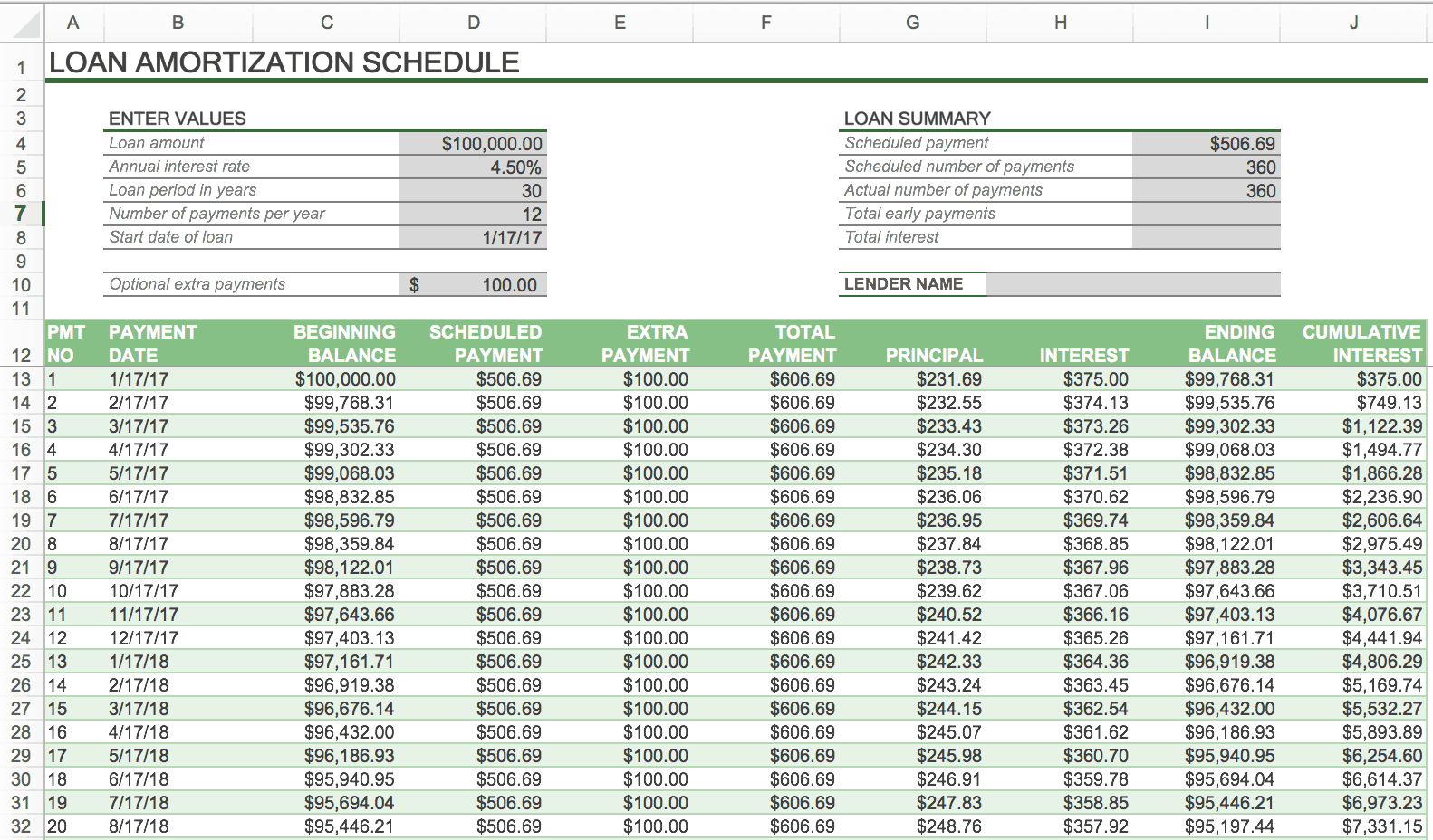
How to make a loan amortization schedule with extra payments in Excel
Hopefully, the amortization schedules covered in the earlier examples are simple to make and adhere to. They do not, however, include a helpful feature that many borrowers would find appealing: making additional payments to speed up loan repayment. We’ll look at how to make a loan amortization schedule with additional payments in this example.
Define input cells
As usual, begin with setting up the input cells. Let’s name these cells as follows in this instance to make our formulas easier to read:
- InterestRate – C2 (annual interest rate)
- LoanTerm – C3 (loan term in years)
- PaymentsPerYear – C4 (number of payments per year)
- LoanAmount – C5 (total loan amount)
- ExtraPayment – C6 (extra payment per period)

Calculate a scheduled payment
In addition to the input cells, we also need one more predefined cell (the scheduled payment amount) for our additional calculations. e. the loan balance due if no additional payments are made This amount is calculated with the following formula:
Please take note that in order to get a positive number as the result, we put a minus sign before the PMT function. We enclose the PMT formula within the IFERROR function in order to prevent errors in the event that some of the input cells are empty.
Enter this formula in some cell (G2 in our case) and name that cell ScheduledPayment. 
Set up the amortization table
Make a loan amortization table using the headers displayed in the following screenshot. Enter a string of numbers in the Period column that start with zero (you can hide the Period 0 row later if necessary).
Enter the greatest number of payment periods that can be entered if you want to create a reusable amortization schedule (0 to 360 in this example)
Pull the Balance value for Period 0 (row 9 in our example), which is the total of the initial loan. All other cells in this row will remain empty:
Formula in G9:
=LoanAmount 
Build formulas for amortization schedule with extra payments
This is a key part of our work. The built-in functions in Excel do not allow for additional payments, so we will have to perform all of the math ourselves.
Note. In this illustration, row 9 corresponds to Period 0 and row 10 to Period 1. In the event that the beginning row of your amortization table is different, please make sure to modify the cell references accordingly.
After entering the following formulas in row 10 (Period 1), repeat the process for each of the subsequent periods.
Scheduled Payment (B10):
Use the scheduled payment if the amount (designated as cell G2) of the scheduled payment is less than or equal to the remaining balance (G9). If not, add the outstanding amount plus the interest from the prior month.
We encase this and all ensuing formulas in the IFERROR function as an additional safety measure. In the event that some of the input cells are empty or contain invalid values, this will stop a variety of different errors.
Extra Payment (C10):
Return the ExtraPayment if the amount (designated as cell C6) is less than the difference (G9-E10) between the remaining balance and this period’s principal; if not, use the difference.
Tip. Simply enter each individual payment amount in the Extra Payment column if your additional payments are variable.
Total Payment (D10)
Add the extra payment (C10) and the scheduled payment (B10) for the current period, that’s all:
Principal (E10)
Return the smaller of the two values—scheduled payment minus interest (B10-F10) or the remaining balance (G9)—if the schedule payment for a given period is greater than zero; return zero otherwise.
Note that the principal only represents the portion of the scheduled payment (not the additional payment!) that is applied to the principal of the loan.
Interest (F10)
Divide the annual interest rate (named cell C2) by the total number of payments made each year (named cell C4), and multiply the result by the amount left over after the previous period if the schedule payment for a given period is greater than zero. If not, return 0.
Balance (G10)
Subtract the principal amount of the payment (E10) and the additional payment (C10) from the balance that remains after the previous period (G9) if the remaining balance (G9) is greater than zero; return 0 otherwise.
Note. During the process, some of the formulas may display incorrect results because they cross reference—not circular reference! Therefore, kindly wait to begin troubleshooting until you have entered your amortization table’s final formula.
If all done correctly, your loan amortization schedule at this point should look something like this: 
Hide extra periods
As stated in this tip, set up a conditional formatting rule to hide the values in unused periods. The distinction is that this time, we fill the rows with zero or empty values for Balance (column G) and Total Payment (column D) by using the white font color:
Voilà, all rows with zero values are hidden from view: 
Make a loan summary
Using these formulas, you can output the most crucial details about a loan as the ultimate touch of perfection:
Scheduled number of payments:
Divide the total number of years by the annual payment amount.
Actual number of payments:
Beginning with Period 1, count the cells in the Total Payment column that are greater than zero:
=COUNTIF(D10:D369,">"&0)
Total extra payments:
Cells in the Extra Payment column should be added up, starting with Period 1:
=SUM(C10:C369)
Total interest:
Columns in the Interest column are added together, starting with Period 1:
=SUM(F10:F369)
Optionally, hide the Period 0 row, and your loan amortization schedule with additional payments is done! The screenshot below shows the final result: 
Amortization schedule Excel template
To make a top-notch loan amortization schedule in no time, make use of Excels inbuilt templates. Just go to File > New, type “amortization schedule” in the search box and pick the template you like, for example, this one with extra payments: 
Next, save the freshly made worksheet as an Excel template so you can use it anytime you’d like.
This is how you use Excel to make a loan or mortgage amortization schedule. I appreciate your time and hope to see you on our blog the following week!
You may also be interested in
- Hi. attempting to update this table to reflect new monthly fees which increases the loan amount rather than additional payments that lower the loan amount Since that the interest rate is applied to the amount borrowed rather than the entire repayment amount, do I just add a minus sign to the additional payment amounts, or is there another way I can accomplish this? Thanks.
- thnks!
- I appreciate you, Svetlana Cheusheva. I used your examples, and they were very effective. Other than that, you provided all the information I needed. I had to look up the defined naming.
- I used the same sample data and followed your tutorial; I learned a lot along the way, too, and got exactly the same results! That’s fantastic! But I also followed another tutorial that I didn’t get from ablebits, and it used PPMT and IPMT along with additional payments. Although the outcomes were comparable, the total interest came to $166. 77 higher than in your example. Although the two tutorials appear to follow the same logic—balance, principle, extra payment—and assume that the extra payment contributes to the principle balance, the outcomes differ. I assume it’s because of what you mentioned in this post, “We will have to do all the math on our own because Excel’s built-in functions do not provide for additional payments,” but I’d love to know why there is a difference. The balance can be found using the following formula: =IFERROR(IF(G9 >0, G9-E10-C10, 0), “”). The formula from the other tutorial is =I10-K10-N10, which is essentially the same as G9-E10-C10. I10 = Starting Balance, K10 = Principal PMT Portion (cell formula is -PPMT(InterestRate/12, Period, Term, Principle (absolute reference))) N10 = Extra Payment. It appears that this is where the differences lie. Could you please clarify?
- I need help putting up the following columns in a loan amortization schedule: 1 Due date (due dates must be spaced one month apart from the date of loan issuance): 2 Payment date 3. Payment amount 4. Accrued interest 5. Principal payment 6. Interest Payment 7. Principal balance 8. Interest balance The following are the schedule’s rules: 1 Since the loans are amortized, interest is assessed on the principal 2 balance as it decreases. Interest is assessed on the principal amount plus the total interest accumulated as of the last due date if a client fails to make payments by the deadline. 3. Repayment is applied first to any interest that has been accumulated, and any remaining funds are used to lower the principal that is still owed. Thank you. Your request is more extensive than what we offer on this blog. There is no one formula that can be used to find this complex solution. I’ll do my best to respond to any specific queries you may have regarding how a function or formula works.
- I’m attempting to construct the schedule with additional payments, but I’m stuck at steps 1 and 2. The instructions for step 1 seem to indicate that we should type “InterestRate” as a hyperlink somehow in cell D2, but in the example for step 2, that cell is blank. Are we supposed to name the input cells as “InterestRate – C2 (annual interest rate)” or “annual interest rate” in cell A2? I’ve tried all of the names, but I can’t get the schedule payment fields or balance to compute. Nevermind. I didnt know about the “Name Box”. Thank you! This instruction just got much easier now that I know that.
- QUESTION. NOT THAT I AM EXCEL EXPERT, I BUILT TABLE ABOVE. NOTICE HOW INTEREST IS COMPUTED IN THE EVENT THAT THE BALANCE IS NOT INCLUDED IN THE FORMULA I TESTED FORMULA BY ADDING 200. 00 TO PAYMENT AMOUNT, BALANCE WAS REDUCED, BUT ALL COLUMNS RETAINED THE SAME INTEREST
- Hi Team, these are really nice schedules. But would you kindly help with a schedule that includes both the initial loan and further borrowings? First loan in year one, followed by loans in years three, four, and five, in that order Thank you Team .
- Hi, I’m looking for a sheet similar to this one that can have 30 cars on it and that displays the information vertically rather than horizontally. Hi there, is there anything similar available? The TRANSPOSE function allows you to convert data from vertical to horizontal. This article might be useful for you: Using Excel’s TRANSPOSE function to convert a column to a row using a formula I must include more information about the moratorium and the additional payment feature in the sample file that has been provided. Can you share the file if it has already been created or provided?
- Please let me know if the loan amortization table is available in Excel. If so, could the loan amortization table be updated client-by-client and automatically adjust for interest rate changes? If so, what does “extra payments” mean? Specifically, “start at payment no,” “extra payment,” “payment interval,” “extra annual payment,” “payment,” “total extra payment,” “variable or fixed rate,” and “impact of interest rate hike on your loan EMI.”
- Making monthly mortgage payments at the end of the month wouldn’t make sense, so why wouldn’t the payments be made at the beginning of the period (using type 1 in the excel PMT calculation)? Since real estate loans are paid back in arrears, the end of the period is appropriate.
- How to add extra payments on non payment due dates?
- My actual annual interest rate is 19, so is there a way to prevent the Annual Interest Rate cell from rounding up? Six percent, and the number is automatically rounded up to 2020 when I enter it into the cell, causing the running balance to be slightly off. Since I’m not very proficient with Excel, I most likely made a mistake. I appreciate your help and information. Hi there, I hope this article on Excel calculation precision can be of use to you. Modify the format of the cell numbers and add more decimal places. I hope it’ll be helpful.
FAQ
How do I make an amortization schedule for a loan?
First, multiply your principal balance by your interest rate to determine amortization. Next, calculate your interest rate for the current month by dividing that by 12 months. Finally, subtract that interest fee from your total monthly payment. The remaining amount is what will be applied to the principal for that month.
Which Excel function is most important when creating an amortization schedule?
In order to create an amortization schedule in Excel, the PMT function is required. It calculates the constant periodic loan payments.
What is the formula for loan sheet in Excel?
The loan amount should be entered into one cell of an Excel spreadsheet. In another cell, enter the loan tenure, making sure to maintain a constant time frame (months or years). Enter the annual interest rate in another cell. Enter “=PMT(interest rate/12, loan tenure*12, -loan amount)” without quotation marks in a new cell.
Read More :
https://m.youtube.com/watch%3Fv%3DQZfMW203v4U
https://www.ablebits.com/office-addins-blog/create-loan-amortization-schedule-excel/